Cellular automata (and related lattice models)
The mathematical notion of automaton indicates a discrete-time system with finite set of possible states, a finite number of inputs, a finite number of outputs, and a transition rule which gives the state at the next step in terms of the state and inputs at the previous step.
A Cellular Automaton applies this notion in parallel to a cellular space, in which each cell of the space is a stateful automaton. The essential components that define a cellular system are:
Cellular space: A collection of cells arranged into a discrete lattice, such as a 2D grid. The space is usually 1D, 2D or 3D, but rarely greater.
Cell states: The information representing the current condition of a cell. In binary CAs this is simply either 0 or 1.
Initial conditions: What state the cells are in at the start of the simulation.
Neighborhood: The set of adjacent/nearby cells that can directly influence the next state of a cell. The most common 2D neighborhoods are:
State transition function: The rule that a cell follows to update its state, which depends on the current state and the state of the neighborhood. It gives the cell state[t+1] as a function of the states[t] of itself and neighbours.
Time axis: The cells are generally updated in a discrete fashion, which may be synchronous (all cells update simultaneously) or asynchronous (cells update sequentially).
Boundary conditions: What happens to cells at the edges of the space. A periodic boundary 'wraps around' to the opposite edge; a static boundary always has the same state, a reflective boundary mirrors the neighbor state.

The CA model was propsed by Stanislaw Ulam and used by von Neumann -- in the 1940's -- to demonstrate machines that can reproduce themselves. Decades later Christopher Langton proposed a more concise self-reproducing CA, which has since been further improved upon using artificial evolutionary techniques:
CAs are not just for exploring this question. Christopher Adami describes CAs as the first "artificial chemistries", since they operate as a medium to research the continuum between the (such as molecules in crystal and metalline structures) and the living (such as cells of a multi-cellular organism). Thus they can be used to model all kinds of information processing and development in biological systems, as well as questions of life's origins. (However the computational cellular systems we will visit are far, far simpler than biological cells.)
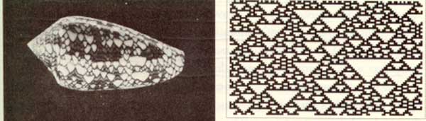
Stephen Wolfram, author of Mathematica, performed extensive research on CAs and uncovered general classes of behaviour comparable to dynamical systems. A commonly referenced example is his 'rule 30', which is a 1D CA displayed below as a stacked trace (history goes down) -- whose pattern is reminiscent of some naturally occurring shell patterns:
Here are some of the well-known 1D rules:
See the Pen 1D Rules: 2019 by Graham (@grrrwaaa) on CodePen.
Wolfram divided CA into four classes, according to their long-term behavior:
- Class 1 - stable. Evolves to homogeneous state.
- Class 2 - cyclic. Evolves to simple separated periodic structures. Local changes to the initial pattern tend to remain local
- Class 3 - chaotic. Any stable structures that appear are quickly destroyed by the surrounding noise. Local changes to the initial pattern tend to spread indefinitely
- Class 4 - complex. Local changes to the initial pattern may spread indefinitely. Wolfram has conjectured that many, if not all class 4 cellular automata are capable of universal computation.
Over here a 3D cellular automaton is taking over Minecraft, and here is a self-replicating computer in 3D.
Conway's Game of Life
The most famous CA is probably the Game of Life. It is a 2D, class 4 automata, which uses the Moore neighbourhood (8 neighbours), and synchronous update. The transition rule can be stated as follows:
- If the current state is 1 ("alive"):
- If the neighbor total is less than 2: New state is 0 ("death by loneliness")
- Else if the neighbor total is greater than 3: New state is 0 ("death by overcrowding")
- Else: State remains the same ("alive")
- If the current state is 0 ("dead"):
- If the neigbor total is exactly 3: New state is 1 ("reproduction")
- Else: State remains the same ("dead")
It is thus an example of a outer totalistic CA: The spatial directions of cells do not matter, only the total value of all neighbors is used, along with the current value of the cell itself. Note also that these rules mean that the Game of Life is not reversible: from a given state it is not possible to determine the previous state.
The Game of Life produces easily recognizable higher-level formations including stable objects, oscillatory objects, mobile objects and objects that produce or consume others, for example, which have been called 'ponds', 'gliders', 'eaters', 'glider guns' and so on.
This CA is so popular that people have written Turing machines and, recursively, the Game of Life in it.
Implementation
If the cells are densely packed into a regular lattice structure, such as a 2D grid, they can efficiently be represented as array memory blocks. The state of a cell can be represented by a number, so an array of integers works well. A way to index this array memory to read or write a cell coordinate will be useful.
In theory the transition rule can be represented as a look-up table, however above a certain number of states and neighbors the size of this table would become astronomical (k states raised to the power of k neighbor states raised to the power of n neighbors; for a 3-state, 3-neighbor system this requires 7 billon rules!), so a procedural implementation is preferable. CAs may use bit-wise operators to implement the transition rules in a hardware-optimized way, but we will use regular if statements for clarity.
One complication is that the states of the whole lattice must update synchronously. That means: when one cell changes, all cells should change. This is not easy to achieve in most computing systems today, which mostly follow instructions one at a time (with only limited parallelism). A naive implementation will thus update cells one at a time, and the neighborhood of a particular cell will contain both 'past' and 'future' states. One way to work around this is to maintain two copies of the lattice; one for the 'past' states, and one for the 'future' states. The transition rule always reads from the 'past' lattice, and always writes to the 'future' lattice. After all cells are updated, either the 'future' is copied to the 'past', or the 'future' and 'past' lattices are swapped, since the future of yesterday is the past of tomorrow.
This technique is called double-buffering, and is widely used in software systems where a parallel process interacts with a serial machine. It is used to render graphics to the screen, for example.
See the Pen 2019 DATT4950 Jan 3 by Graham (@grrrwaaa) on CodePen.
Variations
There are many ways we can modulate this into more complex CA. For example, by allowing more than two states. For example, here is "Brian's Brain":
See the Pen Brian's Brain: 2019 DATT4950 by Graham (@grrrwaaa) on CodePen.
More variations are possible by modulating the basic definition of a CA, some of which have been explored more than others.
Probabilistic/Stochastic CA
In this case the transition rule is not deterministic, but includes some (pseudo-)randomized factors. This can help avoid the CA falling into a stable or cyclic pattern -- at the risk of descending into uninteresting noise.
- A probability can be assigned to each successor state according to the prior states. For example, take a look at the Forest Fire CA below, and try changing the probabilities to see how it behaves:
See the Pen Forest Fire: 2019 by Graham (@grrrwaaa) on CodePen.
- A backround noise can be added, such that from time to time a randomly chosen cell changes state. Try adding background noise to the Game of Life to avoid it reaching a stable or cyclic attractor. But too high a probability and it descends into noise. Try adding a temperature control to control the statistical frequency of such changes. Could something intrinsic to the system determine temperature? Could this vary over space?
- Probabilistic/statistical choices can be combined with other variations below, such as spatially non-homogenous probabilities, statistical rules and neighbourhoods, etc.
Non-homogenous CA
The rule is not the same for all cells / for all time steps. Spatial inhomogeneity can be interesting to simulate different geographies (such as boundaries). The simplest option is to prime the system with inhomogeneous initial conditions, but these differences can quickly dissipate, whereas varying other components of a CA spatially can have more profound results (though, as with randomness, care may need to be taken that these differences do not overly dominate the process).
- Creating unusual neighbourhoods (or simply, non-totalistic ones) can introduce interesting spatial biases to behaviour.
- Special boundary cells in the field may follow different rules from others.
- Some rules may depend on the cell position; perhaps the same CA has different regions using different rules. These can be implemented by changing the function used in the transition rule, or by extending the state set to accommodate the differences. Changing the function is usually easier to implement and understand.
Temporal non-homogeneity can be used to perform a sequence of different filters, or otherwise help to build long- as well as short-term arcs of behaviour.
- The neighborhood selection rules could change over time (also see particle CA below).
- The rules used could alternate between different rule definitions, over a period of N frames. Or certain parameters to rules could cycle over certain periods. Scott Draves' Bomb modulated parameters continuously, with different rule sets picking up the last as their new initial conditions.
- Variations of space/rule/neighborhood could depend on global conditions, such as the overall density of black and white cells, or due to user interactions.
- Other combinations of the above (and below)
One has to be careful though: it could be that introducing these variations is not really different to a slightly more complex, but homogenous, CA.
Asynchronous CA
Rather than updating all cells at once, some other policy of visiting cells to update is applied.
A fixed update policy, such as linear scan or pre-determined path, is orderly, but may introduce artifacts (related to the double-buffering pattern). A randomized, but still fixed, order can still lead to artifacts.
A multi-rate CA (self-clocked) updates each cell according to a clock period that varies from cell to cell. This implies that each cell must have more than one value (one to store the state, one to store the period, one to store the phase) -- or equivalently, that there is more than one cellular grid. The clock period or phase could be affected by that of neighbours'. This may lead to entrainment effects.
- Mobile CA (see below)
- Probabilistic asynchrony (see below)
Mobile CA
A mobile CA has a notion of active cells. The transition rule is only applied to active cells, and must also specify a related cell (such as one of the neighbors) of the current active cell as the next active cell. (This could also be partly probabilistic.)
There could be more than one 'active cell' -- there could even be a list of currently active cells. Non-active cells are then described as "quiescent". But what happens if two active cells occupy the same site?
Langton's Ant
- Langton's Ant is a mobile CA in a 2D, two-state space, with very simple rules:
- At a white square, turn 90° right, flip the color of the square, move forward one unit
- At a black square, turn 90° left, flip the color of the square, move forward one unit
See our JavaScript version:
See the Pen Langton's Ant: 2019 by Graham (@grrrwaaa) on CodePen.
A variation with multiple ants:
See the Pen Multiple Langton Ants: 2019 by Graham (@grrrwaaa) on CodePen.
The original video by Christopher Langton, including examples of multiple ants (and music by the Vasulkas):
Note that Langton's Ant, and other related Turmites, are closely related to the turtle graphics often used for L-systems, which we will return to later in the course.
Termites
Mitchel Resnick's termite model is a random walker in a space that can contain woodchips, in which each termite can carry one woodchip at a time. The program for a termite looks something like this:
- Look at the space just in front of me
- If it is empty, move forward and randomly change direction (random walk)
- Else if it is occupied by a woodchip:
- If I am carrying a wood chip, drop mine where I am and turn around
- Else move forward and pick up the woodchip
Over time, the termites begin to collect the woodchips into small piles, which gradually coalesce into a single large pile of chips.
Particle CA and Lattice-Gas Automata
If the transition rule (or, the set of transition rules as a whole) is careful to preserve a total cell values before and after, it can give the impression of a mass-conserving system, such as modeling the motion of particles and fluids. The elementary 1D traffic CA (rule 184) is a simple particle CA.
Block rule CA
Since mass-preservation can be ensured by considering the neighbourhood before and after each transition, rules are often expressed in terms of a block. For a 2D CA, the simplest block is a 2x2 region (the Margolus neighborhood).

A clever technique to simulate block-based rules is to shift the block grid on each successive frame, such that the even-aligned and then odd-aligned blocks interleave (see wikipedia). Note that a block rule CA does not need to be double-buffered, since block updates do not overlap.
Examples of 2x2 block rule CA are listed here -- many of these are implemented below:
See the Pen Block Rules: 2019 by Graham (@grrrwaaa) on CodePen.
In 1969, German computer pioneer (and painter) Konrad Zuse published his book Calculating Space, proposing that the physical laws of the universe are discrete by nature, and that the entire universe is the output of a deterministic computation on a single cellular automaton. This became the foundation of the field of study called digital physics. Zuse's first model is a 3D particle CA.
A CA-inspired digital physics hypothesis is currently being promoted by Stephen Wolfram, as described in his magnum opus A New Kind Of Science.
Some observations
The block-rule CA especially hints at another interpretation of CA as a pattern-based rewriting system -- a point we will return to later in the course. And in fact, many CA can be understood as the application of pattern-based rewrites, in which a region of space that matches a given template pattern is replaced by a new region with the template's corresponding result (or action).
Clearly, mass-preserving CAs are guaranteed not to dissolve into homogenous final states -- which can alleviate any need for an external limiter to keep the balance -- but this does not mean they won't find a stable or cyclic end. On the other hand, CAs whose rules do not appear to preserve mass can still avoid dissolution into homogeneity.
Note that mass-preservation does not imply that the system is reversible. Reversibility is quite a different property, which states that each output neighbourhood can only be caused by a single predecessor neighbourhood. Some, but certainly not all, particle CAs are reversible.
Particle CA can also use probabilistic rules to simulate brownian motions and other non-deterministic media (but the rules would usually still need to be matter/energy preserving over long-term averages -- i.e. probabilities must balance to preserve mass). Particle CAs can also benefit from the inclusion of boundaries and other spatial non-homogeneities such as influx and outflow of particles at opposite edges to create more interesting gradients or otherwise keep the system away from equilibrium (a dissipative system).
Probabilistic Asynchronous CA
Chooses the next active cell according to a random selection.
The Ising model of ferromagnetism in statistical mechanics can be simulated in a Monte Carlo fashion: Each site (cell) has either positive or negative spin (we can encode that as 0 or 1 value). At each time step, consider a site at random, and evaluate the probability of changing state. If changing state moves the site closer to energetic equilibrium with its neighbors (determined according to the Hamiltonian) of the site), then the change is made. Otherwise, the change is made only with a small probability that is dependent on the energetic difference and overall temperature. Thus at high temperatures, the system remains noisy, while at low temperatures it gradually self-organizes into all sites with equal spin.
[A simplified Ising model on codepen -- try changing the temperature:
See the Pen Simple Ising: 2019 by Graham (@grrrwaaa) on CodePen.
The contact process) model has been used to simulate the spread of infection (and changes of opinion in voting): infected sites become healthy at a constant rate, while healthy sites become infected at a rate proportional to the number infected neighbours (see also the HodgePodge simulation below). This can be extented to multiple states for a multitype contact process.
See the Pen HodgePodge: 2019 by Graham (@grrrwaaa) on CodePen.
Large/unbounded/complex states
The cellular Potts model (also known as the Glazier-Graner model) generalizes probabilistic asynchronous CA to allow more than two site states, and in some cases, an unbounded number of possible site states; however it still utilizes the notion of statistical movement toward neighbor equilibrium to drive change, though the definition of a local Hamiltonian. Variations have been used to model grain growth, foam, fluid flow, chemotaxis, biological cells, and even the developmental cycle of whole organisms.
Note that in this subfield of research, the term cell is used not to refer to a site on the lattice, but to a whole group of connected sites that share the same state. So in modeling foam, a cell represents a single bubble, and is made of one or more sites. Most changes therefore happen at the boundaries between these cells.
Stan Marée used this model to simulate the whole life cycle of Dictyostelium discoideum!
States need not be discrete integers -- in other systems the state could be represented by an n-tuple of values, or a recursive structure allowing unbounded complexity.
Continuous automata
The CAs we have looked at so far are mostly discrete, and this is often evident in the results. But there are several ways in which we can try to approximate fully continuous automata -- and investigate to what extent similar properties or behaviours arise, and whether new properties can arise unique to continuous spaces. At the least, continuous automata are more able to show liquid and diffusive effects. But to proceed, we must consider each of the discrete aspects in turn:
Continuous states: In this case, the states are not discrete (such as 0 or 1) but belong to a continuum (such as the linear range 0..1). We have seen some examples of this already (e.g. HodgePodge). The transition rule can no longer be a simple lookup table, but instead must map continuous ranges and/or functions. Comparators can be used to segment continuous space into ranges, and drive control flow, but the use of control flow implies that the output of the transition rule is still principally discontinuous.
Continuous transition functions: One step further requires that the transition rule be expressible as a purely mathematical function, that is predominantly smooth. That is, all transition rules are combined into a single function, which handles both continuous input and produces continuous output. A sigmoid function, for example, is a continuous input & output function that nevertheless approximates the states of discrete functions.

Another option here is to introduce probabilistic functions. Finding a continuous system whose behaviours persist with the addition of some random noise is tantamount to finding an interesting system that is robust to perturbations -- a useful feature for anything that must interact with the real world!
Continuous neighborhood: Instead of simply considering whole neighbor cells, we may want to apply some kind of weighted average over the surrounding region -- a sampling "kernel". Proper weighting of a kernel can eliminate much of the artifacts due to regular grid spacing.
The kernel could be simply expressed as an inner and outer radius, for example, or an ideal distance with sampling weighted according to a function of distance from this radius.
If radii are not expected to change, then kernel locations and weights can be pre-computed. Nevertheless, continuous neighborhood sampling can easily become processor-intensive. It may also be viable to explore a statistical sampling strategy, selecting each time only a random sub-set of the possible sampling locations to create a cheaper approximation of continuous sampling.
Another option is to apply an intermediate process of diffusion -- i.e. blur -- across the entire space between each application of the transition rule. However it is important that the diffusion kernel is mass-preserving -- that is, that repeated applications of the blur will not make the sum of all cell values greater or lesser.
Continuous time: Instead of simply outputting a new state, change may be spread over time as a differential. That is, what is output from the transition function is an offset to accumulate to the current state.
This offset may also be distributed over a weighted neighbourhood, rather than a single state.
Another possible strategy to explore is delayed application (i.e., spreading the double-buffering over continuous time): maintaining copies of past and future cell states and interpolating between them. This can be used to smoothen the visual output of the CA, and also to support sampling the field at arbitrary points of time between frames.
Smoothlife
SmoothLife uses a discrete grid, but all of states, kernel, and transition functions are adjusted for smooth, continuous values. A disc around a cell's center is integrated and normalized (i.e. averaged) for the cell's state, and a ring surrounding this is integrated & normalized (averaged) for the neighbor state. Cell transition functions are expressed in terms of continuous sigmoid thresholds over the [0, 1] range, and re-expressed in terms of differential functions (velocities of change) to approximate continuous time. Paper here. By doing so, it removes the discrete bias and leads to fascinating results. Another implementaton. Taken to 3D. In effect, by making all components continuous, it is essentially a simulation of differential equations. Here is a great explanation of the SmoothLife implementation, with a jsfiddle demo
Lenia
Lenia continues in the spirit of SmoothLife, and has been extensively explored & documented to identify over 400 different organisms, occuping distict environmental niches (different physical constants), with various locomotive patterns catalogued, etc.
- Paper
- Code
- Winner in Virtual Creatures Contest, GECCO 2018, Kyoto
- Honorable Mention in ALife Art Award, ALIFE 2018, Tokyo.
Reaction Diffusion
The reaction-diffusion model was proposed by Alan Turing to describe embryo development and pattern-generation (Turing, A. The Chemical Basic for Morphogenesis.); it is still used today in computer graphics (Greg Turk's famous paper). RD systems and other differential equation systems can be approximated using continuous automata.
One approach to simulating RD using CA is the Gray-Scott model, as described in Pearson, J. E. Complex Patterns in a Simple System. A browser-based example is here.
There is a wonderful archive of this model at this webpage, including many great video examples of the u-skate world, and even u-skate in 3D.
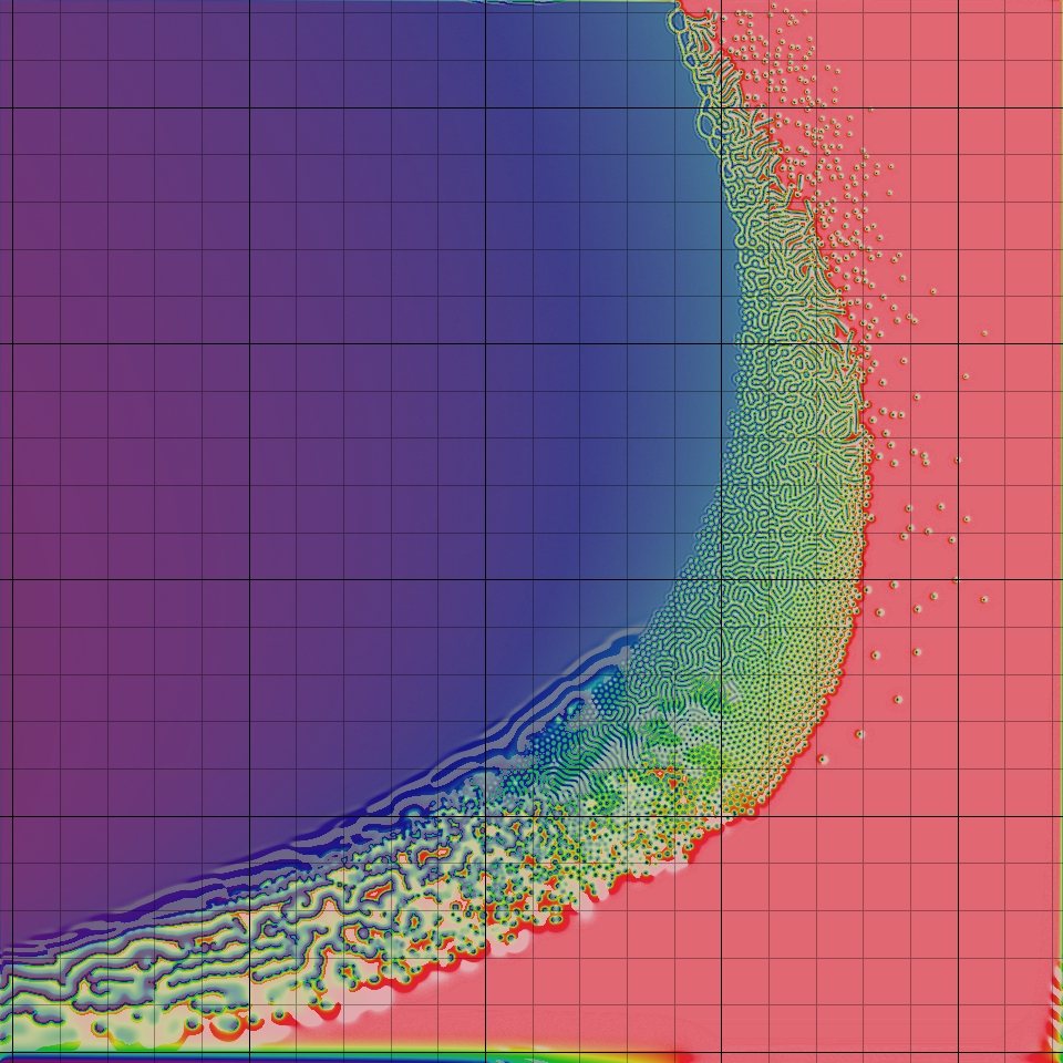
Here is this model at a lower resolution using our starter kit:
See the Pen Reaction Diffusion: 2019 by Graham (@grrrwaaa) on CodePen.
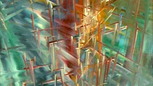
Some of these systems share resemblance with analog video feedback (example, example), which has been exploited by earlier media artists (notably the Steiner and Woody Vasulka).
Spatial transformation systems
Apart from smooth sampling, we can also introduce interesting behaviours by transforming the space itself as it is sampled. Different indexing rules (such as affine transformations of coordinate space) can be used to impart non-local symmetries and behavior. Different rules (or different neighborhood specifications) can be run in parallel on the same shared data.
Such transformations can effectively create non-standard neighbourhood rules.
Transformations can be global, or vary according to local field variations. For example, this beautiful viscous fingering shadertoy uses continuous values and sampling along with a spatial rotation, where the rotation applied is a result of the field's curl) (the infinitesimal rotation) at a particular point.
Ima Traveller

Artists Driessens & Verstappen created a recursive cellular system (exhibited in the artwork IMA Traveller) which appears to show an endless zoom; as the whole field appears to expand, each cell periodically subdivides into four daughter cells, following one of several rules to vary the color. Cells outside the viewpoint are thrown away. The effect is an infinitely expanding landscape or journey, which can be partially navigated by the gallery visitor. See the info link. Driessens & Verstappen: Ima Traveller
Ima traveller (1996) is interactive computer software for exploring an infinite universe. It enables you to make a journey into a space that is being created in real time. This space develops in the direction you are moving into, so there is no end to it. You travel forward in a smooth motion, you can drift in all directions, but you can never go back to where you came from. You are zooming in on a surface of infinite size, never reaching any boundaries.
This work has inspired discussion by several critics, including Mitchell Whitelaw and Jon McCormack and Alan Dorin.
Multi-scale systems
Several cellular systems can be coupled together at different scales.
- Perhaps each cell of a macro-CA is itself an entire micro-CA world. Or several CA can overlap with different spatial relationships.
- Higher- and lower-level systems could progress at different rates (or statistical frequencies).
Jonathan McCabe's cyclic multi-scale Turing patterns, and a commentary by Mitchell Whitelaw. The implementation is described in this paper.
It starts with a straightforward reaction-diffusion system:
- Diffusion is simulated by averaging the continuous cell values over small (activator) and large (inhibitor) radii; if the the smaller (activator) concentration is greater than the larger (inhibitor) concentration, increase the cell value by a small amount; otherwise decrease.
- After running the rule over all cells, the entire field is normalized (to ensure the minimum cell value is zero and the maximum cell value is 1).
Since this creates structure at a single spatial scale, it can be elaborated by super-imposing several models at different spatial scales (different small and large radii). Or, by changing the radii dynamically over time (as in Greg Turk's famous paper). McCabe's system uses several pre-defined scales, but selects which scale to apply for a particular cell according to which one currently shows the least local variation.
Additionally, his system does not measure all cells within a radius; instead it selects cells at the radius distance and certain angular directions, creating cyclical symmetries in the result. For example, 3-fold symmetry may be used at a smaller scale, and 9-fold symmetry at a larger scale.
Multi-way CA & parallel histories
In certain CA variants, more than one substitution could be valid to undertake. We have seen how some CA simply choose randomly between options, while Monte Carlo systems consider two or more options and take the one with the highest entropy. In a sense, for a brief moment, these systems follow two parallel histories, and then choose which one to discard. But there is no reason why we can't follow two (or more) histories for a little longer than a single step, nor to limit our decision-making to an energetic/entropic basis. We may return to this idea when exploring evolutionary systems, which present a similar parallelism.
Wolfram also explored 'multi-way' CA executions, in which all possible histories for a given state are explored, considering their long-term evolutions, and in particular exploring which rules lead to exponentially more universes, which tend to stabilize, and which ultimately lead to the same results.